APPENDIX F: ADDITIONAL CONSIDERATIONS
This appendix describes two additional types of quality control procedures that may be of interest: Classification Accuracy and Completeness. At this time, it is difficult to recommend appropriate thresholds for acceptance criteria. However, ground classifications should be achievable with >90% accuracy.
Classification Accuracy
Points in a LIDAR dataset can be classified through semi-automated and in some cases automated processes. Typical classification categories for point clouds include terrain, vegetation (low, medium, high), buildings, etc. Note that ground filtering/vegetation removal algorithms tend to perform much better with airborne LIDAR data compared to Mobile or Static LIDAR techniques due to the look angle. In addition to geometric accuracy, in the case of a classified point cloud, one would need to evaluate the classification accuracy to determine levels of omission and commission. For example, a point that is classified as ground but is really vegetation could lead to problems in DTM creation, depending on the robustness of future algorithms. Further discussion of this topic is beyond the scope of this document.
The classification accuracy of a point cloud can be determined by manually classifying points in several representative sample sections and comparing them to the classifications provided by the service provider. Statistics can then be developed on how well the points were classified for each category, into a Confusion Matrix (Figure F-1) showing the quantities and types of mis-classifications. Ideally, the matrix would be a diagonal matrix with 100% along the diagonal, showing that all data points were classified into the appropriate category.
Figure F-1: Example of a confusion matrix comparing predicted versus actual classification accuracies by categories.
Data Completeness
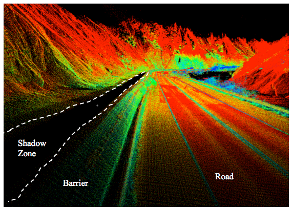
Another consideration is a completeness factor describing the frequency of data gaps. While parts of the scan data will meet resolution requirements, there will be many cases where there will be data gaps (i.e., shadows, occlusions) due to visibility constraints (Figure F-2). The acceptable quantity and locations of these gaps will be important to consider when certifying the final deliverables. A simplified metric can be obtained in 2D by comparing the area covered by scan data (meeting a sampling threshold) to the total desired coverage area. For more sophisticated procedures on calculating completeness, see Yoo et al. (2010). These procedures, however, require 3D models of the scene to be created, which will not always be available. Hence, due to that reason and difficulties in implementing these methods with existing software we do not describe them herein.
On the road surface or objects that are orthogonal to the MLS, completeness >90% should be easily achievable. However, the completeness quality will degrade with distance from the scanner trajectory because the shadow from a small object blocking the scanner will enlarge with distance. Further, small data gaps from moving objects passing in front of the scanner are less of a problem than larger gaps from static objects (e.g., parked vehicles). To help counteract this, collection should be done during low traffic periods. Implementation of a rolling slowdown behind the scanner can eliminate problems with vehicles creating data gaps. Multiple passes will also help fill in these data gaps.


